
The Triumph of the Quantity Theory of Money, 2020–2025
How far can a simple theory take you during a once-in-a-century monetary shock? Pretty far, it turns out.

An Overview of the Theory
In intro macro we teach the quantity theory of money as a way to think about the impact of changes in the money supply on the average price level over the long run:
M v = P Y,
where
M: money supply, typically measured using M2
v: velocity of money, or the average number of times each dollar is spent per year
P: average price level in the economy, typically measured using the CPI
Y: real GDP
The quantity theory of money is less a grand theory than an accounting identity. On the left, we have the total amount of dollars circulating in the economy (M) multiplied by the number of times each dollar is spent per year (v), which is equal to nominal GDP. On the right, we have real GDP (Y) multiplied by the average price level (P), which is also equal to nominal GDP. Since there is only one value of nominal GDP, both the left and right hand sides must yield the same result.
We can measure the money supply (M), average price level (P), and real GDP (Y), but we cannot observe the velocity of money (v) directly. The quantity theory of money is thus used to impute the value of v such that both sides of the equation match. In other words, v is chosen to make the identity hold.
The key insight comes from rewriting the equation in growth rates (by taking logs and differentiating with respect to time):
gM + gv = gP + gY,
where gx is the growth rate of variable x. Note that gP is the growth rate of the price level, or inflation.
In the short run, money creation can stimulate demand. But in the long run, printing money cannot generate sustained growth in real GDP. So the first assumption we make is that money growth does not cause real GDP growth in the long run.
The second assumption is that the velocity of money is stable over time (i.e., gv= 0). This assumption is not trivial. After the 2008–09 financial crisis, many expected rapid money growth to generate inflation, but velocity collapsed instead. The same thing happened during the first few months of the Covid-19 recession. But in this case velocity recovered relatively quickly back to its pre-Covid level, making the assumption of stability a reasonable simplification for this period.
Under these two assumptions, the theory implies that in the long run, money growth equals inflation plus real GDP growth:
gM ≈ gP + gY.
That’s the scaffolding we’ll use to evaluate what happened since 2020.
Implications for Monetary Policy
To fix ideas, suppose the money supply is constant (gM = 0). Then if real GDP grows, more goods are being produced but there are no new dollars to buy them, so the average price level must fall (gP < 0). In other words, we get deflation.
Most modern central banks actively try to avoid deflation by growing the money supply (gM > 0). If the Fed sets gM equal to gY, then real GDP can grow while the price level stays flat (gP = 0).
In practice, the Fed targets 2% inflation. The theory tells us how to hit it: set money growth equal to real GDP growth plus 2%.
gM = gY + 2%
Real GDP growth has averaged about 3% per year in the postwar period. So money growth of about 5% per year is consistent with hitting the 2% target. It really is that straightforward.
It seems like every day there are new data releases about the labor market, inflation, or real GDP growth. These headlines distract central bankers and market watchers from what matters most for achieving stable prices: the growth rate of the money supply. As Milton Friedman preached, “Inflation is always and everywhere a monetary phenomenon.”
Application: Covid-19 Recession and Recovery
When the pandemic hit, the Fed slashed rates to zero and bought Treasuries and MBS in unprecedented quantities. The result: the money supply exploded. The quantity theory tells us those dollars had to show up somewhere.
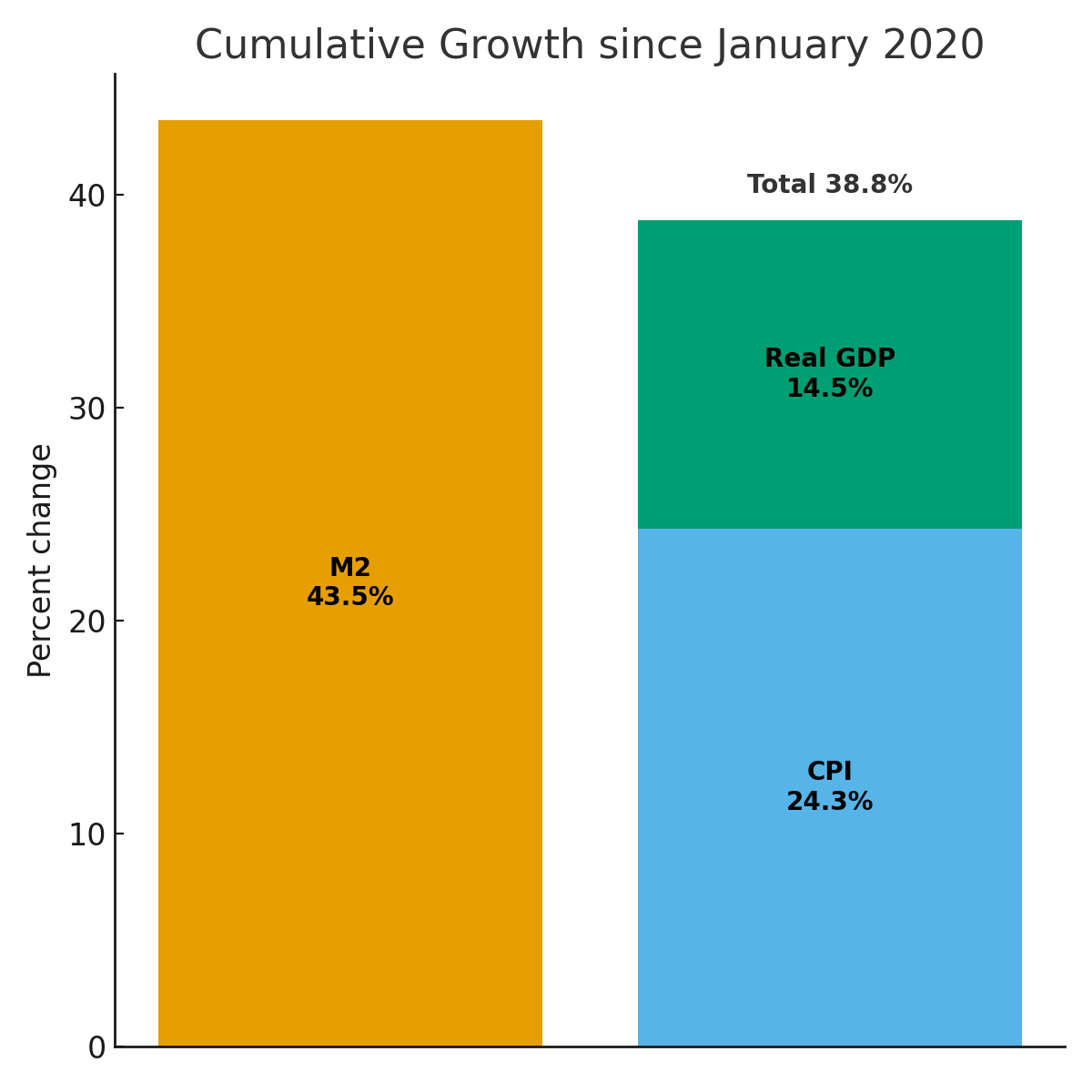
As shown in Figure 1, between January 2020 and July 2025 the money supply increased by 43.5% (M2SL). Over this same period, real GDP rose by just 14.5%. According to the theory, the price level should rise by:
gP = gM – gY = 43.5% – 14.5% = 29%
I call this potential inflation: how much inflation is in the pipeline if money and real growth stop here.
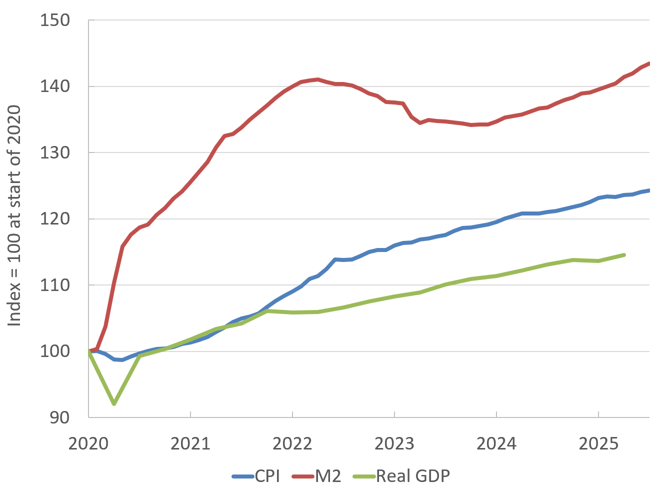
How does that compare to actual inflation? Between January 2020 and July 2025, the CPI increased by 24.3%. Not the full 29%, but close. Importantly, velocity today is about where it was in early 2020, meaning money growth must show up eventually in real GDP growth or inflation.
So what do we learn?
The quantity theory, on its own, explains the inflation we experienced since the Covid-19 pandemic. No need to invoke supply bottlenecks or “greedflation.” Inflation was never going to be transitory; it was baked in by money growth, waiting to be realized.
There is still some potential inflation left out there. The theory predicts 29%. We’ve seen 24.3%. That leaves about 4.7% unaccounted for. Faster growth could soak it up (see Figure 2). But unless velocity slows again, that wedge will eventually show up somewhere, either in higher prices or more output.
Implications for the Fed Now
We enter late 2025 with solid growth and low unemployment, but new tariffs are starting to push up import prices, which may kick off the potential inflation still remaining in the system.
Over the last 12 months:
Money growth (M2): ~4.8%
Inflation (CPI): ~2.7%
Real GDP growth: ~2.1%
Through the lens of the identity, this mix is close to target. With a 2% inflation goal and plausible real growth of 2–3% ahead, money growth of about 5% is consistent with keeping inflation near target absent new easing. If real growth accelerates inflation should moderate toward 2%.
If money growth is already stable, easing now risks another round of persistent inflation. The Quantity Theory of Money suggests the Fed should proceed with caution.
What does this mean in practice for monetary policy going forward?
Anchor nominal growth. The Fed should keep money growth consistent with 2% inflation plus real growth.
Watch broad money. If M2 growth runs well above 5% while tariffs are raising import prices, expect inflation pressure to rebuild. As I argued in The Fed Should Ignore Tariff Induced Inflation, the Fed should not respond to a one-off tariff shock by either tightening or easing financial conditions. If the Fed does ease, it won’t be a one-off shock; it is a setup for persistent inflation.
Let QT keep running quietly. Passive balance sheet runoff is an important tool the Fed should use to restrain money growth without constant headlines.
Conclusion
The past five years show the enduring power of a first principles framework. The quantity theory of money was enough to predict that the surge of money printing would lead to inflation. It reminds us that over the long run, money growth and real GDP growth together determine the prevailing amount of inflation. For the Fed, the task now is simple in principle but not in practice: keep money growth aligned with real capacity, and inflation takes care of itself.
Notes and Sources
AI tools were used to help transform raw data into figures and to edit prose; all calculations are straightforward to reproduce from the cited sources.
If you enjoyed this mildly efficient and occasionally rational take on the Quantity Theory of Money, consider subscribing below. We’ll continue exploring markets and models, revealing mildly surprising truths. No hot takes; just thoughtful ones.

About the Author: Seth Neumuller is an Associate Professor of Economics at Wellesley College where he teaches and conducts research in macroeconomics and finance. He holds a Ph.D. in economics from UCLA. His Substack is Mildly Efficient (and Occasionally Rational) where he explores topics in finance and macro from first principles, cutting through complexity with clear, grounded analysis.